• Reminder about airfoils

• Airfoil behavior

• Reynolds and Mach numbers

• Aerodynamic of the blade

• Combined constraints

Summary

Geometric parameters of an airfoil are defined in general by :

• the chord connecting the trailing edge to the leading edge (this straight line is the longest distance between the trailing edge and the leading edge area),

• the upper line expressed as a percentage of the chord along Y axis versus X axis location,

• the lower line expressed as a percentage of the chord along Y axis versus X axis location,

• the mean camber line which is drawn halfway between the upper and lower lines (mean algebraic value between upper and lower line). The resulting camber is characterized by its max value and its related location (a symmetric airfoil has a null camber),

• the thickness line expressed as a percentage of the chord is the algebraic difference between Y values of upper and lower line. The max thickness and its location helps to define the airfoil properties,

• the leading edge radius which is the curvature giving the leading edge shape,

Resulting from these definitions, an airfoil gets a camber if the upper line curvature is more pronounced than the lower one, generally at the front part of the airfoil (convex mean line). An airfoil gets reflexed when, at the rear part, the curvature of the upper line is not so pronounced than the lower one (concave mean line). The combination of the two gives a mean line in « S » with an inflexion point (« S » airfoil).

Example of « S » airfoil : mean line is convex at leading side and concave at trailing side:

Summary

The airfoil behavior depends on the different modes of operation of the enclosing boundary layer when it moves at a defined velocity through the air. The boundary layer is characterized by an intense shearing of air particles from the airfoil surface (at the airfoil surface particles are stuck by viscosity : velocity to airfoil is null, max velocity regarding the incoming airflow) up to where the particles reaches the velocity of the incoming airflow (max velocity to the airfoil, null velocity regarding the incoming airflow). The followings can be considered :

• The laminar region around the leading edge. Air particles move in a relative order with a minimum friction. Then the laminar flow gets thicker up to the transition point before growing turbulent. The laminar layer is highly fragile and unstable ; it is also very thin, in the order of 1/10mm.

• The transition point located between laminar and turbulent regions which position is essentially variable and unstable at low Reynolds number, generally close to 50% of the chord. This point is sometimes considered as a region.

• The turbulent region in which air particles are agitated, generating much more friction than in laminar region. Similarly the turbulent flow gets thicker up to the separation point. Surprisingly, the turbulent particles make the flow more stable than the laminar one. The turbulent flow thickness is larger than the laminar one. Also the thickness depends on the Reynolds number : the lower it is the thicker are the laminar and turbulent flow.

• The separation point ends the turbulent region and indicates the separation of the boundary layer from the airfoil shape. The downstream velocity is then inverted, meaning air particles come against the stream to fulfill the empty location due to separation. Lift falls down while drag increases a lot : these are the stalling conditions.

• The stagnation point corresponds to the flow line which velocity gets null in contact with the leading edge (null velocity and max pressure). In other words the stagnation point is at the contact of the leading edge with a perpendicular plane to the line that splits the flow upper from the flow lower. This line is not straight but curved upward before reaching the stagnation point.

The graphic below shows the velocity distribution of an Eppler 201 airfoil at an angle of attack of 6 degree 

It is usual to call velocity from infinity (V) by designating the velocity and the direction of airflow to the airfoil, in practice at a point distant of several chords from the airfoil. Bypassing the airfoil, the flow is subject to acceleration/deceleration and its related velocity (v) varies considerably. At the stagnation point the related velocity (v) is null. Then following the ratio (v/V) on the upper surface, values in the order of 2 can be reached in the first percent of the chord (considerable acceleration generated by change of direction and strong suction) then it decreases steadily toward 1 close to the trailing edge. On the lower surface the flow acceleration is smooth and stabilizes its ratio (v/V) below 1 (velocity lower than the velocity from infinity). The surface enclosed between upper and lower velocity is proportional to the lift. In case the lift is null, the two curves overlap in such a way the enclosed surfaces come to neutral.

Air velocity variations within the thickness of the boundary layer are not the same in laminar region and turbulent region : it is steeper in the turbulent region (velocity gradient higher producing more friction).

As long as the boundary layer is laminar or turbulent the lift coefficient (Cl) is not affected. It is only the case if there is separation of the boundary layer from the airfoil, resulting in the stalling effect.

The target consist in keeping the boundary layer in laminar rate as far as possible on the upper side to take advantage of low friction. When increasing the attack angle, stalling conditions are created : the separation point at the trailing edge appears traveling on the upper surface towards the leading edge, while the stagnation point moves lightly backwards on the lower surface (up to a tens of % of the chord). To fulfill the laminar rate conditions, it is required that the airfoil shaping manages at best possible the kinetic energy provided by the upper airflow to make it easy to reach the trailing edge (at this point the flow velocity is about 85% of the velocity from the infinite). If flow lines take off the airfoil surface there is separation of the boundary layer and drastic increase of the drag. For some airfoil, depending on their upper curvature, separation might take place and followed by a reattachment of the boundary layer : a bubble is so created enclosing a turbulent mode (drag +++) and sometimes announcing the stall. Some techniques have been implemented to re establish the laminar rate by sucking the bubbles. Similarly bubbles at the upper leading edge can occur, if the curvature radius is low, under the strong acceleration of air particles combined with the centrifugal force.

 
Drag coefficients increase dramatically at low Reynolds numbers, with important instability and uncertainty of magnitude. It becomes quite risky to work out something under the level of 100 000. Considering a set of various airfoils at « low Reynolds number » and « human flight » classes, the values of Cdmin are quite similar and the difference is made mainly on the Cl available range with Cd values close to the minimum. Although it seems obvious, it’s better to remind that the best Cl/Cd ratio is reached when the Cd is still low and the Cl near its maximum. To make it clear, at Reynolds number of 100000 the best Cd values cannot get down as low as 0.01 while the best Cl/Cd ratios hardly get over the bar of 80. At this little game, airfoils with medium camber are generally at the top of performances. Take care however, airfoils themselves are not alone to do the job : for example, at given lift and rotor diameter, it is required to shorten the chord or the tip speed as long as you increase the camber but the Reynolds number decrease... dilemma ! Candidate airfoils are numerous and if one were really above the others everybody would know ! In fact there is no unique solution for a given target in efficiency. Sorry, but compromise is what you get to deal with. The way you operate an airfoil is at least as important as the airfoil itself. The commitment is based on two aspects : define what you want to get out of the airfoil, define what are your operating conditions, both aspects being interactive.

Summary

Summary

• The angle between the chord axis and the driving plane is designated pitch angle (q) «Ò». This is a mechanical angle managed by the control system. q is generally lower than 20 degrees and, in some case, depends on the radius (twisted blade).

H
We can also define a reference pitch angle at a particular chord location. This reference helps to define the pitch control system and is compulsory in case of twisted blades. It is recommended to choose the tip pitch angle as the reference.
 

• The attack angle (a) is the angle between the chord axis and the resultant relative wind axis. This aerodynamic angle represents an incidence angle of the airfoil in the close environment of the rotor.

H
It is considered as effective attack angle (a_e), when it includes not only the Froude wind but also the ½ blade induced wind. This reduces the angle value.
 

• The relative wind angle (b) is the angle between the driving plane and the axis of relative wind.

H
It is considered as effective relative wind angle (b_e), when it includes not only the Froude wind but also the ½ blade induced wind. This increases the angle value. One should notice that :q  =  a + b.

Projections

Drag and lift forces result from the airflow circulation through the rotor in accordance with the previous definitions. The drag is carried by the relative wind axis and the lift is perpendicular to it.

As drag axis and lift axis are inclined of the relative wind angle, it is necessary to project both lift and drag onto the rotor axis on the one hand and on the driving plane on the other hand to get the resulting axial lift and the resulting drag. The resulting axial lift «Ò» is the combination of the lift projections plus the drag projection on the rotor axis (this reduces the lift). The resulting drag is the combination of the drag projections plus the lift projection on the driving plane (this increases the drag). The resulting drag is at the root of the axial torque«Ò» and of the required power under the form of specific power «Ò» expressed in W/kg (specific to the lifted mass unit).

One should notice that the axial lift is in deficit regarding the lift itself and the resulting drag is in excess regarding the drag itself. This corresponds to inevitable losses : less lift and more drag are obtained. Also, it can be seen that the greater the angle of attack and the relative wind angle are, the more losses appear ; this being more significant when the lift is important compared to the drag. In fact it is of current use to consider the resulting drag as the sum of a so called shape drag (specific to airfoils and viscosity constraints) and an induced drag (resulting from the lift projection). To generate a given lift, at a given chord and rotor diameter, a cambered airfoil gets this results at low angles, causing a lift less inclined and less induced drag. This is an important factor that allows to minimize the losses but only a complete computation «Ò» helps to find the optimal solution. Don’t forget however that the more « power consuming » parameter is the rotation speed that impacts the power by its square value.

Summary

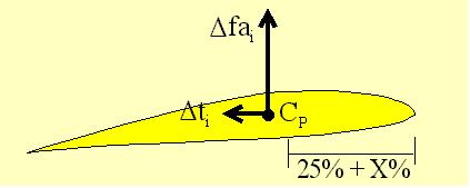
Center definitions

The gravity center (C_G) is the internal point of a blade that enables to keep the blade balanced whatever its orientation is. It is at this point that gravity and centrifugal forces applies. Knowing this point enables to calculate the blade moment (static moment) which is the product of the distance of the gravity center to the rotor axis by the blade mass.

The gravity center (or at least its projection on the upper surface) can be easily determined : for that, protect the foreseen area with a sticker and balance the blade (lower side up) on a cutter edge via two oblique orientations. The junction of the two marks provides a very good estimate of the X, Y location.

Don't forget that when analyzing a blade station per station, each station has a mass and a center of gravity by itself, located in general at the same distance from the leading edge than the resulting center of the complete blade only in case of rectangular top view. The natural location of the center of gravity for a blade made with homogenous material is in the 40% region from the leading edge (at least for current cambered airfoils).

The aerodynamic center (C_A)  of any airfoil is the point located by convention at 25% of the chord from the leading edge. At this point the moment coefficient is practically independent from the angle of attack (or at least this is the point where it is the less dependent). This coefficient value is either null for a symmetrical airfoil or negative for a cambered airfoil. Airfoil data give the coefficient value implicitly linked to the aerodynamic center.

The lift center (C_P) «Ò» of any airfoil is the point where the resulting moment is null and consequently the resulting aerodynamic force only applies at this point. In case of symmetric airfoils the aerodynamic center and the lift center are merged. In case of cambered airfoils, the lift center is generally back to the aerodynamic center and all the more as the camber is important (from 25% for symmetrical airfoils it can move back to 50% for some cambered airfoils).

The lift center can be derived from the aerodynamic center applying a conversion to the system of forces (see the related window hereafter). In case of cambered airfoils, the lift center travels forward when increasing the pitch angle so progressively coming closer to the aerodynamic center.

The rotation center (C_A) is the mechanical point round which the blade rotate (feathering). The longitudinal or span wise axis goes through this point. Its position has no influence on the blade twist and is of little effect on the resulting moment of the blade and also about the control constraints. 

For any airfoil and to minimize the twist effect (further explained), it is ideal that the average location (span wise) of lift center merge with the gravity center. This common location is then at 25% for symmetric airfoil (lead insertion at the leading edge to get the balance) and can be in the order of 40% for cambered airfoils (no lead required).

According to the picture, it can be seen that the combination of lift forces (Dfa_i) and centrifugal forces (Dfcn_i), caused by conicity, generates a twist moment if C_G and C_P are separated. This moment is upward (then positive) if the lift center C_P is located ahead of the gravity center C_G and the twist increases the pitch progressively up to the tip. In principle this not completely satisfactory, but acceptable if it is limited. In this case, the constraints are of « retention » type as much as the pitch is deviated from neutral (contrary to the "return to flat" action). In some cases a null resulting moment can be reached but most of the time the blade is subject to a residual twist which depends on the twist coefficient of its structure. The resulting twist is in general lower than a degree and should be taken into account in the computation of the rotor lift.

In conclusion :

• In case of cambered airfoil, it is better to manage the gravity center location lightly ahead of the lift center so that the resulting moment be rather downward, even null. The airfoil choice and the material distribution along the chord is important to get this result « naturally » (otherwise lead inclusion is required for balance). Our glass/carbon composite blades are naturally balanced without lead. The simulation «Ò» helps to know the resulting twist at given conditions of operation.

• In case of symmetric airfoils, it is required to merge the gravity center and the lift center to get a null resulting moment. This condition is generally obtained with addition of lead. It is interesting to notice that this result is independent from operating conditions and particularly from conicity.